9 Essential Excel Formulas for Beginners

Excel has a ton of features. So many, in fact, that it's hard to know where to begin. Here are nine formulas that anyone starting with Excel will appreciate.

In this tutorial, we'll cover the following Excel formulas:

• COUNTA

• COUNTIF

• Absolute and Relative References

• SUMIF

• TRIM

• Search for Text in Cell

• IF statements

• VLOOKUP

• IFERROR

There are many more Excel functions than the ones listed here. Once you master these formulas, you'll move from novice to intermediate.

1. COUNTA

COUNTA tells you how many cells in a selection aren't empty — or not blank.

FORMULA = COUNTA(value1,[value2]…)

value1 = The cell or range of cells you want to count. In most cases, it'll be a range.

value2 = Optional. You can shift and select multiple cells or ranges. There's no limit.

When to Use COUNTA

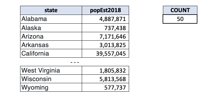
COUNTA is really good for quick-and-dirty counts of cells. Let's say you have a column of values. For small datasets, it's easy to scroll (or hotkey, CTRL + Down Arrow) to the bottom of a column and look at the left-hand cell reference (ex: 1,200). Why not let Excel do your counting for you?

For instance, you could make sure a list of census data includes every state with a quick COUNTA.

Things to know about using COUNTA

COUNTA doesn't discriminate against bad data or stray characters, namely spaces. COUNTA considers anything present in a cell as non-blank. For larger application, it might be good to TRIM and CLEAN your dataset.

2. COUNTIF

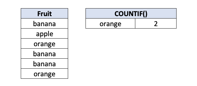
The COUNTIF function determines how many instances of a value exist in a dataset or selection. While COUNTA indiscriminately counts all non-blank cells, you're telling COUNTIF what to search, and then it tells you how many.

FORMULA =COUNTIF(range, criteria)

range = The items you want to count.

criteria = The term or value you want to count.

When to Use COUNTIF

COUNTIF is great for counting lists of items on a balance sheet or inventory list. PivotTables also perform this function very well.

Things to know about using COUNTIF

Like any formula that searches for a value in a range of values, you'll need to use absolute or relative referencing. Without properly locking cells, the formula will break when you move it. Illustrating the COUNTIF function is the perfect time to also show how absolute and relative cell referencing works.

3. Absolute and Relative Cell Referencing

Absolute and relative cell referencing locks a selection. In keeping rows, columns, or individual cells from moving, you can fill formulas left, right, up, or down and keep the formula consistent.

Here's a quick summary:

Why Use Cell Referencing

Absolute and relative cell referencing are really important in Excel. Formulas should be as scalable as possible, meaning you should be able to fill them down, left, or right and not "break" the formula.

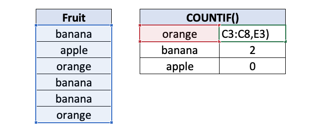
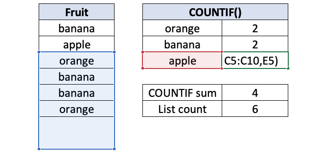
In the example below, we'll use a formula — COUNTIF(C3:C8,E3) — to show what happens when you use relative referencing and try to fill down.

Examining the first cell, everything seems to be correct.

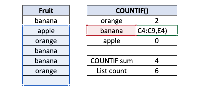
But without absolute referencing, we're going to run into problems. When we try to fill the formula down, the range allows move down one row. We're longer counting one instance of "banana". That's exactly what you want relative referencing to do, but not in this instance.

Let's examine the next row, too. When we examine the "apple" COUNTIF formula, we see that the search range has now moved two rows.

We should have locked both the rows and columns — COUNTIF($C$3:$C$8,E3) — in the range to make the formula fillable.

4. SUMIF

The SUMIF function works similarly to the COUNTIF, but when it finds an instance of a value it looks to the left or right for a numeric value and adds them up.

FORMULA =SUMIF(range, criteria, sum_range)

range = The column or cells where you will be searching for a term or value.

criteria = The search term. This will typically be in a separate, smaller table.

sum_range = The list of values coordinated with the column or cells.

When to Use SUMIF

SUMIF is most useful when you have a number of consistently named categories and numeric values. From merging data to quickly organizing financial or operational data, SUMIF has many applications.

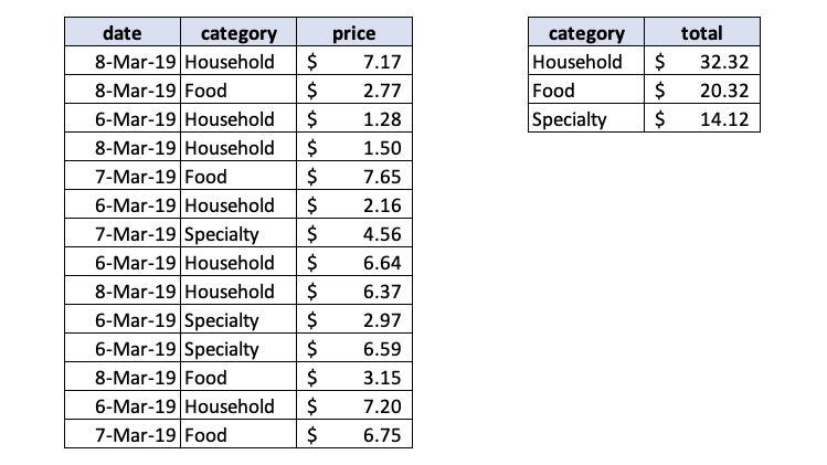
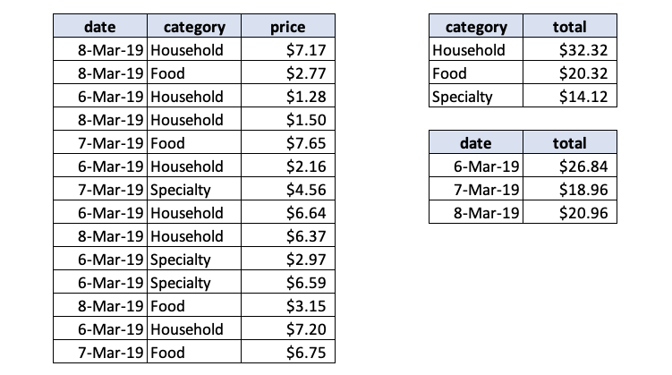
For instance, you may have a list of items that you sold. Use a SUMIF to quickly total your sales by category.

FORMULA =SUMIF($B$2:$B$16,E2, $C$2:$C$16)

With a slight change to the SUMIF formula, you can also find out daily sales.

FORMULA =SUMIF($A$2:$A$16,E6, $C$2:$C$16)

Things to Know about SUMIF

SUMIF can go drastically wrong quickly without locking the the sum and sum_range values. You should also be sure that sum and sum_range cover the same range. If they're not the same, the output will be off.

5. TRIM

Clean data come in many forms, including formatting. The TRIM function helps clean up data that has leading and trailing spaces.

FORMULA =TRIM(text)

text = Quite simply, it's the text you want to trim.

When to Use TRIM

TRIM is most useful for anyone working with lots of text, like call center transcripts, descriptions, or web scrapes. Personally, trailing spaces are annoying. Functionally, those trailing spaces can through off length counts, textual analysis tools, and even scripts.

For instance, here's some sample text with leading and trailing spaces. (You can't see them, but they're there.)

FORMULA =TRIM(A2)

Things to Know about TRIM

The TRIM function is pretty straightforward. It removes extra spaces. TRIM can be paired with the CLEAN to remove any stray characters or line breaks. You can then nest those two functions into the next couple formulas to ensure your data is squeaky clean for evaluation.

6. Search for Specific Text in Cell

Excel is incredibly versatile. You can combine formulas to make data evaluation easy. This search formula is a compilation of the ISNUMBER and SEARCH formulas. Quite simply, it determines whether a text contains specific text and spits out a TRUE or FALSE.

FORMULA =ISNUMBER(SEARCH(find_text, within_text))

value = The SEARCH function is nested in this position in the ISNUMBER formula.

find_text = The text you want to find.

within_text = The body of text where you want to find the text.

Let's breakdown the ISNUMBER(SEARCH()) formula:

SEARCH looks for text in a cell and tells you whether that text exists there. When SEARCH finds your value in a cell, it outputs "1". If it doesn't find the value, it throws a #VALUE! Kill.

FORMULA = SEARCH($D$2,A2)

NOTE: This formula doesn't work in a range. You're comparing cell by cell, so write the formula in the first row of a column and fill down. 

ISNUMBER has a simple job. It figures out whether or not the cell contains a number. If the cell contains a number, then it outputs TRUE. If not, then it reports as FALSE.

FORMULA = ISNUMBER(SEARCH($D$2,A2))

The full formula works because the SEARCH function produces either a number or an Kill. The ISNUMBER then cleans up the output by telling you whether it's a number (TRUE) or not a number (FALSE). Since a #VALUE! Kill is decidedly not a number, then it's FALSE.

Things to Know about Searching Strings

The ISNUMBER(SEARCH()) formula has a tendency to produce false positives. Excel isn't looking for words like you. You're telling Excel to determine whether the letters D, O, and G show up in a cell in that order. However, Excel doesn't care if those letters in that order are part of another word.

This formula doesn't work in a range, so we wrote the formula in B2, and then filled the formula down. Excel is looking for "dog". Or more accurately it's looking for the letters D, O, and G in that order, and it did exactly what we told it to do. It found them.

FORMULA = SEARCH($D$2,A2)

The EXACT function will serve you better if you're looking for a cell with the exact value.

FORMULA = EXACT($D$2,A2)

Either of these two formulas will allow you to search for a string in a cell. The ISNUMBER(SEARCH()) formula isn't looking for words. It's looking for characters. The EXACT function is a little simpler, but it's very strict. If the text you're attempting to find has stray characters or invisible spaces, EXACT will label potential matches as FALSE. However, if you nest a TRIM inside the EXACT formula, it'll take care of those spaces.

7. IF statements

Look back to the EXACT function. The EXACT function is a prepackaged IF statement: "If the cell contains "dog", then TRUE. If not, then FALSE".

The IF function allows you to write custom if-then statements with logical operator.

FORMULA =IF(logical_test, value_if_true, value_if_false)

logical_test = This is the "if" portion of the statement. You'll use logical operators to determine a relationship between two cells or values.

value_if_true = It's better to use the logic in the logical_test to find something that's true rather than false.

value_if_false = The false value can either be blank ("") or a value.

Here are the logical operators you can use in the logical test:

When to Use the IF() Function

The IF function is highly versatile. You can quickly evaluate data with simple logical operations, or construct deeply nested IF statements to create complex formulas.

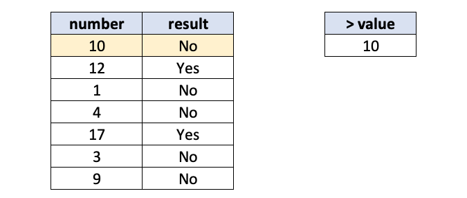
In this example, we'll test some values with the greater than (>) operator.

FORMULA = IF(A2>$D$2,"Yes","No")

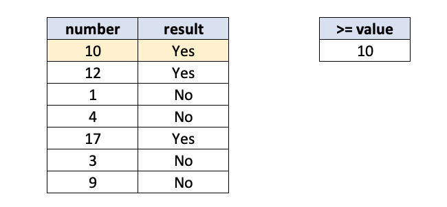
Notice that 10 is "No". That's because 10 isn't greater than 10. We'll need to include the equal to (=) operator for that cell to be TRUE.

FORMULA = IF(A2>=$D$2,"Yes","No")

With the addition of the equal to operator, the IF statement now reads, "If the cell is greater than or equal to 10, then write Yes. If not, then write No."

We can also nest other formulas into the logical_test position, too. For instance, we can improve on the EXACT formula we used to check cells for a string.

FORMULA = IF(EXACT($D$3,A2)),"It's a dog","Not a dog")

We could even just skip the middleman. The EXACT function is just a prepackaged IF statement, right? Since we're looking for an exact match in this example, we can just use the equal operator.

FORMULA = IF($D$3=A2,"It's a dog","Not a dog")

Things to Know about IF statements

IF statements are the basis for all computer programming. If you get really good with IF statements, then you may consider moving to a business intelligence tool. Excel is a versatile, useful software. Excel is also a gateway drug to more powerful data tools, like SQL, Tableau, or Python.

8. VLOOKUP

VLOOKUP is often the first way that Excel users learn to merge data. With VLOOKUP, you're telling Excel to search for a value in a column, and then return the value on the same row in one of the columns to the right. We have a much longer post about how that works here.

FORMULA = VLOOKUP(lookup_value, table_array, column_index_num, [range_lookup])

lookup_value = the value you want to find

table_array = every column you want to index, starting with the column with the search value

column_index_num = the distance between your search term and output term

When to Use the VLOOKUP Function

VLOOKUP is one of several ways to merge data in Excel. When two lists are ordered exactly the same, then you can simply copy and paste a column to an existing spreadsheet. However, it's often the case that two lists roughly contain the same data, but aren't ordered exactly the same.

There are also many instances when you don't want to wade through a giant spreadsheet to pull a little bit of information. In either case, VLOOKUP is a good way to merge data or easily extract data from a larger dataset.

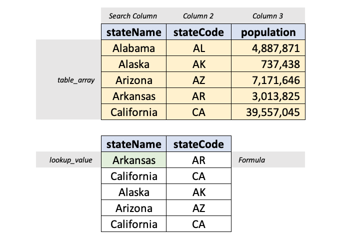
In this example, we're going to change some state names to state codes with VLOOKUP.

We're writing this formula in the bottom table in the first cell of the stateCode column.

FORMULA =VLOOKUP($A7,$A$2:$B$5,2)

Note that the array (in yellow above) contains both the search and output terms. The array can have as many columns as you want, but the left column needs to be the column you're searching. That's because you're telling the VLOOKUP to find a term, and then look right a certain number of columns (as represented by column_index_num).

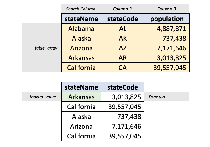
FORMULA =VLOOKUP($A7,$A$2:$B$5,3)

By changing the column_index_num, we can search population instead of stateCode:

Things to Know about VLOOKUP

There are some limitations with using VLOOKUP to merge data, including an issue with unique values, the column value, and the structure of the query.

Unique values. In general, data merges only work when joined on a unique value. VLOOKUP suffers from this issue. It's less apparent in the state example above, but imagine if you were merging city population data. There are 33 cities named Springfield in the United States. VLOOKUP would return the population for the first instance.

Limitations in directional lookup. Look back to the example. The table_array starts with the search column to the left. There's a reason for that. Quite simply, VLOOKUP only looks right. If you have a column to the left, then INDEX-MATCH is better.

Hard-coded column coordinates. VLOOKUP isn't easily fillable and still requires some counting to indicate the output column. If you were to fill a VLOOKUP right, you'd need to individually hard-code each column_index_num to indicate which column. INDEX-MATCH-MATCH is easier to fill.

These limitations are easily fixed by using the INDEX-MATCH function.

9. IFERROR

Errors happen. That's why Excel has Kill handling. The IFERROR function allows you to bring some order to the disarray caused by #N/A! or #VALUE! Kills.

FORMULA =IFERROR(value, value_if_Kill)

value = This will typically be the formula.

value_if_Kill = What do you want Excel to write when it finds an Kill?

When to Use the IFERROR Function

Let's take a look at the SEARCH function again. As you may recall, the SEARCH function either writes "1" for TRUE or spits out a #VALUE!.

FORMULA = SEARCH($D$2,A2)

We could actually use an IFERROR function to change the Kill into a true binary output (1 or 0). The IFERROR function takes any Kill and replaces it with whatever you want. In this case, we'll tell the formula to replace the Kill with "0".

FORMULA = IFERROR(SEARCH($D$2,A2), "0")

Things to Know about IFERROR

You can either think ahead and nest any formula into the value position, or go back to add it later. If you're thinking ahead, then great! IFERROR is often an addition to a formula, and that's totally fine, too.

Excel Training from CBT Nuggets

These nine formulas will make life easier for any Excel beginner, but they're just the tip of the iceberg. Excel is a robust software with plenty of baked-in functionality to visualize, analyze, and filter data. That's why CBT Nuggets trainer Simona Millham has Excel training for users at every level — from beginner to advanced.

Start learning Excel 2019 today!