Microsoft Excel Tips to Make Your Life Easier

Microsoft Excel is packed with a lot of powerful features. At times it can seem intimidating to use. But knowing shortcuts can help get more comfortable with the product and save you time. Discover how to use Excel more efficiently with this collection of tips from CBT Nuggets trainer Simona Millham.

Want to learn even more about Excel? Check out her Microsoft Excel 2019 training at CBT Nuggets.

Microsoft Excel Tech Tips

• Cell Styles are a great way to save and transfer a custom number format. Click the More button on the Styles gallery on the Home tab. Then choose to Create a New Style and be sure to include your custom number format. That's saved with the workbook, but you'll also notice a Merge Styles option, which allows you to bring in Cell Styles from other open workbooks.

• When you have a list of Excel data, click in it somewhere and choose Format as Table from the Home tab. It applies some pretty formatting, yes, but more importantly, it gives you a Table Tools tab on the ribbon with lots of useful options.

• When you format an Excel list as a Table from the Home tab, it knows you want to be able to see your column headings when you scroll. See how the A, B, C column headings have been replaced with the table headings?

• Have you ever lost the grey gridlines around a cell? That's because the cell fill is set to White rather than No Fill.

• You'll probably already know that you can type ' before a number to format it as text. This is useful, for example, if you need to keep the 0 at the beginning for a phone number or something. But what if you've got a list of phone numbers already entered that are missing zeros? The answer is to apply a custom number format.

• You may know that if you type "January" in a cell, you can use Excel's fill handle to continue the pattern. But you can also create your own lists. Type the list, select it, go to File, Options, Advanced, and scroll down to General and click Edit Custom Lists. Click Import, OK, and try it out.

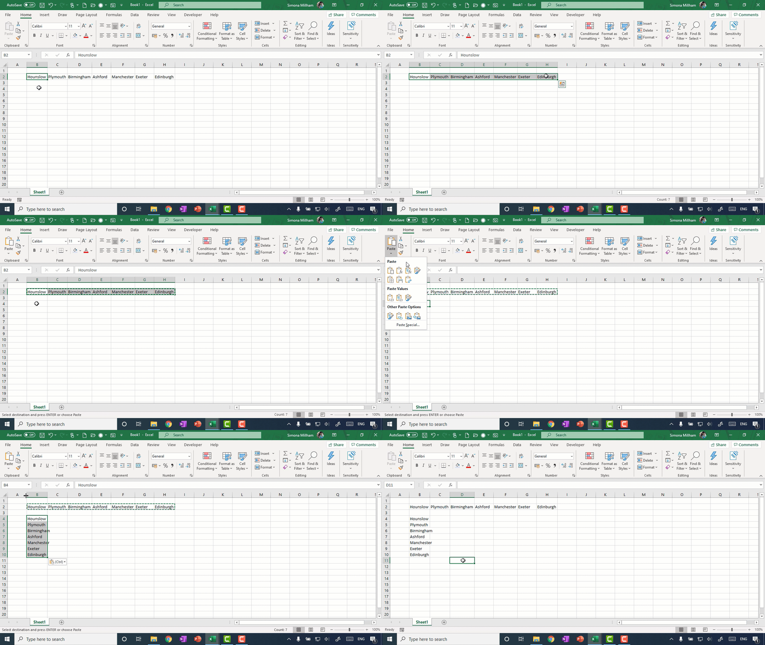
• Do you wish your list of data was in a row rather than a column or vice versa? Copy the cells, click where you want the new list to start, and click the bottom half of the Paste button. Look for the "Transpose" option or just press "T" — and you're done!

• There are some great pre-prepared templates available for you to choose from in Excel. Choose File, New, and if required, search for what you're looking for. You can use them to learn different ways to use Excel.

• Want to change defaults in Excel such as the default number format or header and footer? First, create your ideal blank workbook with the required number format or whatever, and save it as a template called book.xltx in your XLSTART folder.

• Use the Split button on the View ribbon tab to create different window panes that scroll independently.

• If you have cells on one sheet that change when you update figures on other sheets, you might find the Watch Window useful. Click the cells you want to keep an eye on, choose Watch Window from the Formulas tab, and click Add Watch.

• For an instant PivotTable, click in your list of Excel data, go to the Insert tab, and choose Recommended PivotTables. Select the option that looks most useful and bingo!

• Get Excel to read out what you've just typed. Right-click on your Quick Access Toolbar, choose the customize option, display the Commands Not in the Ribbon list, and then find the Speak Cells on Enter button. We imagine this would be highly amusing to switch on for some unsuspecting colleague.

• If you have historical time-based data, try out the new Forecast Sheet option on the Data ribbon tab in Excel 2016!

• If you want to create a PivotTable from more than one Excel list, you can. Just make sure that you tick the box to add the data to the Data Model, which means you'll be able to see ALL the tables in your workbook in the field list. So, when you try to use one, you'll be prompted to create a relationship.

• Does anyone remember in older versions of Excel that the default was 3 sheets in a new workbook? Now it seems to be 1, but you can change this by going to File, Options, and then General.

• Sure, if you want to learn more about an Excel function, you can click "Help on this function" in the Insert Function dialog box, but if you want to browse a list of functions with examples, to potentially uncover some gems, have a look here.

• Try out the Find & Select button on the Home tab. We especially like using this to select all formulas on a sheet.

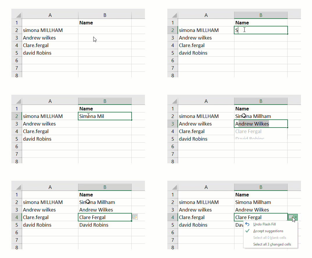
• Use Flash Fill rather than the text functions to tidy up your data. Just type the data as you wish it had been inputted and let Flash Fill do the rest!

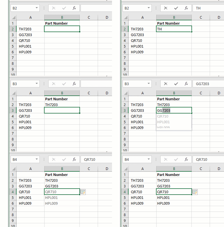
• With Flash Fill, there's no need to use the TRIM function to remove those odd spaces at the beginning of your imported data. You can just type the data as you wish it had appeared —and let Flash Fill do the rest!

• With keyboards getting smaller and smaller, here's a useful tip for navigating your Excel list. Double click the bottom edge of the active cell to get to the bottom of the list and top edge to get to the top.

• You can compare and merge different versions of a Shared Workbook, but you need to add the Compare and Merge Workbooks button to your Quick Access Toolbar. Please note that this tip comes with an official disclaimer about the use of the Share Workbook option on the Review tab, but if you've used it successfully before, you'll find Compare and Merge useful!

• Slot alternative figures into your spreadsheet using the Scenario Manager to see how it affects your calculations. Select the changing cells, go to the Data tab, click What-If Analysis, and choose Scenario Manager. Then create a scenario for each set of figures you want to slot in. As an added bonus, add Scenarios to your Quick Access Toolbar to quickly switch between them. Right-click on the toolbar, choose Customize, and look for Scenarios from the Commands Not in the Ribbon list.

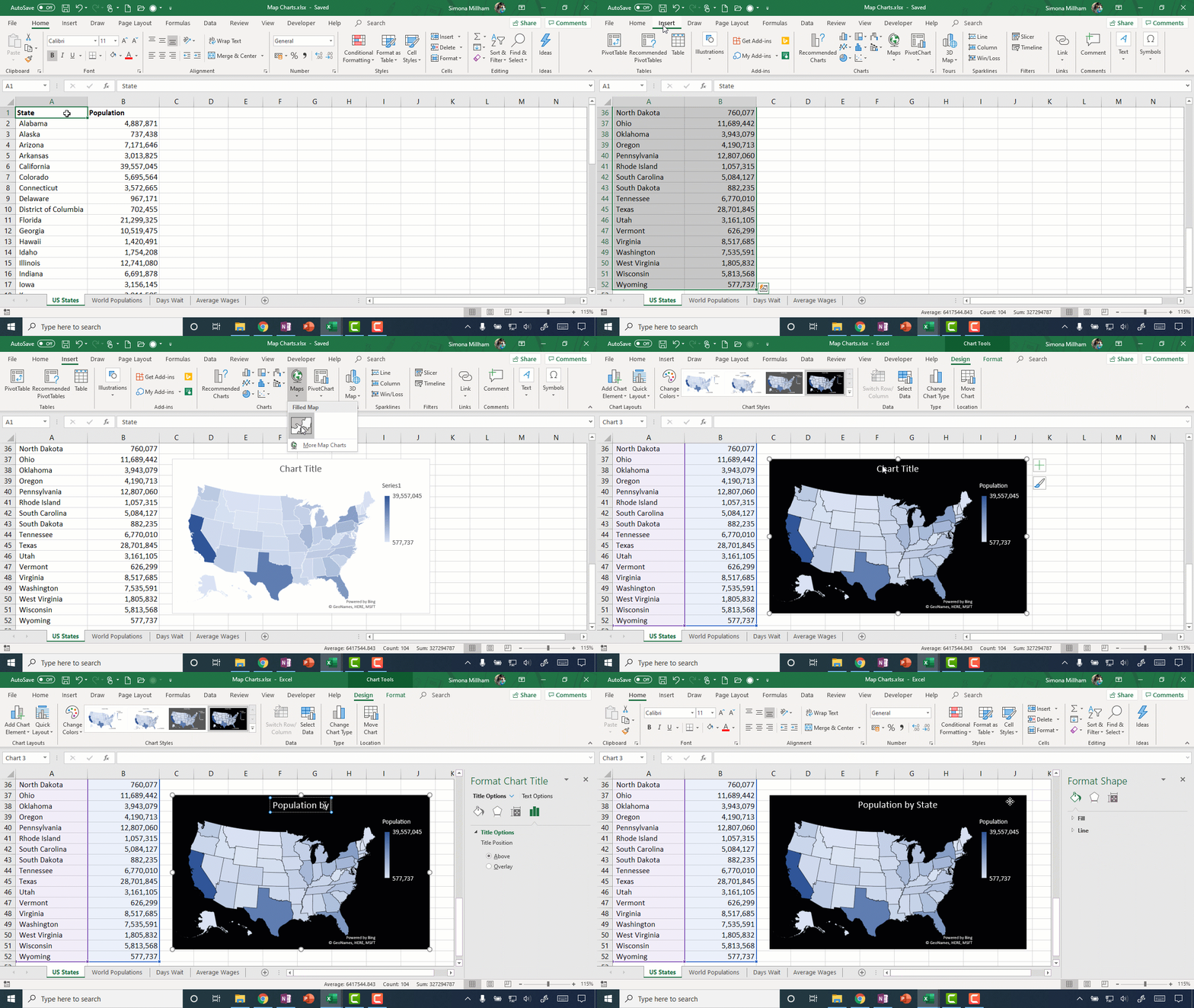
• Have you tried Excel's Map Charts? They're a great option if your data has a geographical element. Find them on the Insert ribbon tab.

• The next time you want to show how many people have done something, how much money something costs, how many products you've shipped, or how much time something takes, try Excel's People Graph. It's really neat! Find it in the Insert menu for Excel 2013 and 2016.

• Oh my goodness, as if six new chart types wasn't enough for Excel 2016, another one has arrived! Find the new Funnel chart in the Waterfall or Stock chart category.

Keyboard & Mouse Shortcuts

• One of my favorite keyboard shortcuts is using CTRL+Page Up and CTRL+Page Down to switch between sheets.

• To enter the same figure into a group of cells, select the cells, type the number, and press CTRL+Enter.

• Press CTRL+SHIFT+7 to add a border around selected cells.

• You're probably used to doing this with a right-click on the row heading, but you can press CTRL+9 to hide a row. To unhide, select cells that span the hidden one and press CTRL+SHIFT+9.

• Press CTRL+0 as a quick way to hide a selected column.

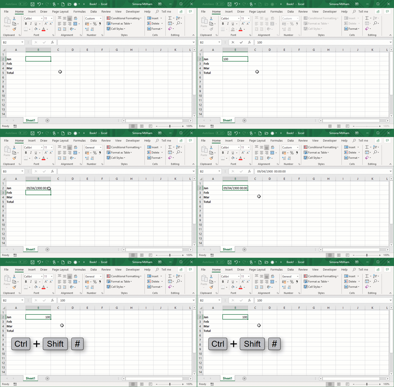
• Have you ever got stuck in some strange number format in Excel? Just press CTRL+SHIFT+# to reset the cell to a general number format.

• Press CTRL+D or CTRL+@ to repeat the contents of the cell above. You'll be surprised how often you use this command.

• Press CTRL+SHIFT+L to turn the sorting buttons on and off in your lists. Simona says: "I actually discovered this by mistake. I mistyped CTRL+SHIFT+; to insert the current time in my timesheet — and found myself turning on the sorting buttons instead!"

• Press CTRL+Spacebar to select a column, or SHIFT+Spacebar to select a row.

• Press CTRL+Tab to switch between open workbooks.

• If you ever need to enter the same information in the same place on multiple sheets, then you can select them and do this all in one go. CTRL+Click the sheet tabs you want to group (or click and SHIFT+Click a range) and get typing.

• To quickly show all formulas on your Excel spreadsheet, press CTRL and then that funny key just to the left of your 1 key, . CTRL+

… What IS that key called?! I'll just call it "that" key. Anyway, try it!

• Select a row or column and press CTRL SHIFT +to insert another row or column.

• Press SHIFT+F2 to insert a comment.

• Press the F4 function key to put the dollar signs into your formula for your absolute cell references. This is much easier than trying to type them in. Keep pressing F4 to toggle through fixing the cell, the column, or the row.

• You can press F9 instead of Enter to input the result of the formula rather than the formula itself. Select the bit you want to evaluate in the formula bar and press F9. Press Escape to return to the full formula.

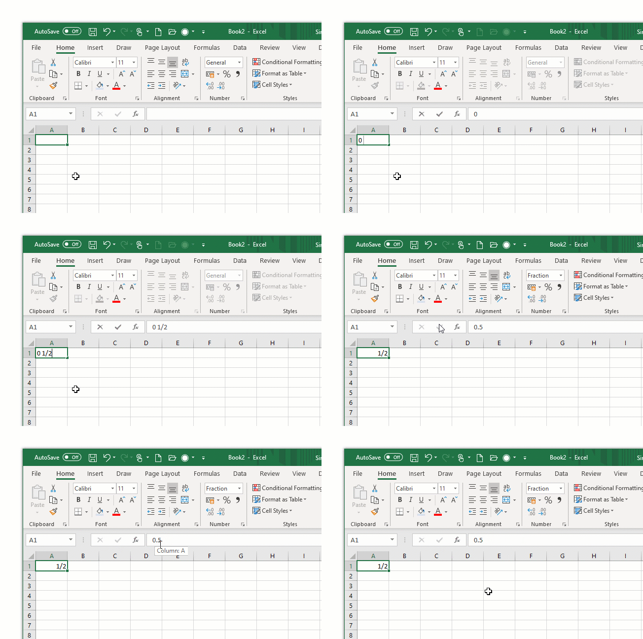
• To enter a fraction, type 0, press the spacebar, and type the fraction — including the slash. Excel will display the value as a fraction and store the decimal value.

• Select the block of cells you want to enter data in, and then use the Enter key to move through the selection in columns or Tab to move in rows. This is more efficient than using the arrow keys!

• If you need to fill weekdays only, use your RIGHT mouse button while you click and drag on the Fill Handle, which is the blob on the bottom right-hand corner of the active cell.

• Press ALT+Enter to start a new line within the same cell. This is useful if the Wrap Text button alone doesn't put the line breaks in quite the right place.

Learn more

For more tips like this, follow Simona on LinkedIn. Start a free week with CBT Nuggets to check out Simona's training for popular tools like Microsoft Word and Skype for Business.